
Learning from Demonstrations with High-Level Side Information
Proceedings of the Twenty-Sixth International Joint Conference on Artificial Intelligence. Main track. Pages 3055-3061.
https://doi.org/10.24963/ijcai.2017/426
Keywords
- Robotics and Vision: Task learning, learning from demonstration, Adaptive control
- Planning and Scheduling: Markov Decisions Processes
- Machine Learning: Reinforcement Learning
- Agent-based and Multi-agent Systems: Formal verification, validation and synthesis
Abstract
We consider the problem of learning from demonstration, where extra side information about the demonstration is encoded as a co-safe linear temporal logic formula. We address two known limitations of existing methods that do not account for such side information. First, the policies that result from existing methods, while matching the expected features or likelihood of the demonstrations, may still be in conflict with high-level objectives not explicit in the demonstration trajectories. Second, existing methods fail to provide a priori guarantees on the out-of-sample generalization performance with respect to such high-level goals. This lack of formal guarantees can prevent the application of learning from demonstration to safety-
critical systems, especially when inference to state space regions with poor demonstration coverage is required. In this work, we show that side information, when explicitly taken into account, indeed improves the performance and safety of the learned policy with respect to task implementation. Moreover, we describe an automated procedure to systematically generate the features that encode side information expressed in temporal logic.
- [Abbeel and Ng, 2004] Pieter Abbeel and Andrew Y Ng. Apprenticeship learning via inverse reinforcement learn- ing. In Proceedings of the twenty-first international con- ference on Machine learning, page 1. ACM, 2004.
- [Albert and Anderson, 1984] A. Albert and J. A. Anderson. On the existence of maximum likelihood estimates in lo- gistic regression models. Biometrika, 71(1):1, 1984.
- [Argall et al., 2009] Brenna D Argall, Sonia Chernova, Manuela Veloso, and Brett Browning. A survey of robot learning from demonstration. Robotics and autonomous systems, 57(5):469-483, 2009.
- [Babes et al., 2011] Monica Babes, Vukosi Marivate, Kaushik Subramanian, and Michael L Littman. Ap- prenticeship learning about multiple intentions. In Proceedings of the 28th International Conference on Machine Learning (ICML-11), pages 897-904, 2011.
- [Baier et al., 2008] Christel Baier, Joost-Pieter Katoen, and Kim Guldstrand Larsen. Principles of model checking. MIT press, 2008.
- [Bertsekas et al., 1995] Dimitri P Bertsekas, Dimitri P Bert- sekas, Dimitri P Bertsekas, and Dimitri P Bertsekas. Dynamic programming and optimal control, volume 1. Athena Scientific Belmont, MA, 1995.
- [Bloem and Bambos, 2014] Michael Bloem and Nicholas Bambos. Infinite time horizon maximum causal entropy inverse reinforcement learning. In Decision and Control (CDC), 2014 IEEE 53rd Annual Conference on, pages 4911-4916. IEEE, 2014.
- [Bobadilla et al., 2012] Leonardo Bobadilla, Oscar Sanchez, Justin Czarnowski, Katrina Gossman, and Steven M LaValle. Controlling wild bodies using linear tempo- ral logic. In Robotics: Science and systems, volume 7, page 17, 2012.
- [Boularias et al., 2011] Abdeslam Boularias, Jens Kober, and Jan Peters. Relative entropy inverse reinforcement learning. pages 182-189, 2011.
- [Dvijotham and Todorov, 2010] Krishnamurthy Dvijotham and Emanuel Todorov. Inverse optimal control with linearly-solvable MDPs. In International Conference on Machine Learning, pages 335-342, 2010.
- [Fainekos et al., 2005] Georgios E Fainekos, Hadas Kress- Gazit, and George J Pappas. Temporal logic motion plan- ning for mobile robots. In Robotics and Automation, 2005. ICRA 2005. Proceedings of the 2005 IEEE International Conference on, pages 2020-2025. IEEE, 2005.
- [John, 1994] George H John. When the best move isn't op- timal: Q-learning with exploration. In AAAI, page 1464.
- [Kress-Gazit et al., 2011] Hadas Kress-Gazit, Tichakorn Wongpiromsarn, and Ufuk Topcu. Correct, reactive, high-level robot control. IEEE Robotics & Automation Magazine, 18(3):65-74, 2011.
- [Kupferman and Vardi, 2001] Orna Kupferman and Moshe Y Vardi. Model checking of safety proper- ties. Formal Methods in System Design, 19(3):291-314, 2001.
- [Macglashan and Littman, 2015] James Macglashan and Michael L Littman. Between imitation and intention learning. In International Conference on Artificial Intelligence, pages 3692-3698, 2015.
- [Neu and Szepesvári, 2007] Gergely Neu and Csaba Szepesvári. Apprenticeship learning using inverse rein- forcement learning and gradient methods. In Proceedings of the Twenty-Third Conference on Uncertainty in Arti- ficial Intelligence, UAI'07, pages 295-302, Arlington, Virginia, United States, 2007. AUAI Press.
- [Ng et al., 2000] Andrew Y Ng, Stuart J Russell, et al. Algo- rithms for inverse reinforcement learning. In Icml, pages 663-670, 2000.
- [Pnueli, 1981] Amir Pnueli. The temporal semantics of concurrent programs. Theoretical computer science, 13(1):45-60, 1981.
- [Ramachandran and Amir, 2007] Deepak Ramachandran and Eyal Amir. Bayesian inverse reinforcement learning. In IJCAI 2007, Proceedings of the International Joint Conference on Artificial Intelligence, Hyderabad, India, January, pages 2586-2591, 2007.
- [Ratliff et al., 2006] Nathan D Ratliff, J Andrew Bagnell, and Martin A Zinkevich. Maximum margin planning. In Proceedings of the 23rd international conference on Ma- chine learning, pages 729-736. ACM, 2006.
- [Wolff et al., 2012] Eric Wolff, Ufuk Topcu, and Richard Murray. Optimal control with weighted average costs and temporal logic specifications. In Proceedings of Robotics: Science and Systems, Sydney, Australia, July 2012.
- [Ziebart et al., 2008] Brian D Ziebart, Andrew Maas, J. An- drew Bagnell, and Anind K Dey. Maximum entropy in- verse reinforcement learning. In National Conference on Artificial Intelligence, pages 1433-1438, 2008.
References were extracted automatically from the PDF and may contain errors.
Full text extracted automatically from the PDF; figures, tables and equations may differ. The PDF is the version of record.
1 Introduction
Learning from demonstration [Argall et al., 2009], also referred to as imitation learning or apprenticeship learning [Abbeel and Ng, 2004], aims at learning a policy to implement some task, using samples of an expert's behaviors as demonstrations. There is a wide range of applications of learning from demonstration in robotics, such as navigation and manipulation tasks.
One common approach to learning from demonstration is inverse reinforcement learning (IRL) [Ng et al., 2000], in which the agent relies on rewards to interpret the expert's behaviors. The environment is modeled as a Markov decision process (MDP) with known transition dynamics.
∗This work was supported in part by AFRL # FA8650-15-C2546, DARPA # W911NF-16-1-0001, ARO # W911NF-15-1-0592, NSF # 1651089 and NSF # 1550212.
Ufuk Topcu
University of Texas at Austin utopcu@utexas.edu
Given the environment MDP and expert's demonstrations as trajectories, IRL recovers a reward function and constructs policies based on the estimated reward function. Formulations of IRL in the literature differ primarily in their interpretation of expert demonstrations, or the "similarity" between the expert's policy and desired policies expressed in terms of rewards. Some common assumptions are, for example, that both the expert's policy and all desired policies are optimal [Abbeel and Ng, 2004; Ratliff et al., 2006; Ramachandran and Amir, 2007; Dvijotham and Todorov, 2010]; or the expected total rewards of output policies should match the sample mean of total rewards of trajectories in demonstrations [Ziebart et al., 2008; Boularias et al., 2011; Bloem and Bambos, 2014].
Although human experts can directly provide low-level demonstrations to implicitly specify the learning task, it is usually beneficial to explicitly indicate high-level task requirements, which we naturally rely on to assess the performance of the learned policies. A high-level task can be "grasp an object without touching anything else," or "obey traffic lights and road signs while driving from A to B," which may not be sufficient to encode all desired properties of an ideal policy, but is crucial to the task performance. Existing IRL methods do not infer underlying high-level tasks and thus the agent's behavior at newly visited states may not satisfy the actual task requirements.
In this work, we join the strengths of high-level task requirements and demonstrations and formalize the problem of IRL with high-level side information. Given task specification as a co-safe Linear Temporal Logic (LTL) formula, and a collection of optimal expert demonstrations consistent with the task specification, we describe a learning framework that recovers both a reward function, as well as a deterministic finite automaton (DFA), which together guarantee a quantitative level of probability that the learned policy will satisfy the task. Crucially, the addition of an LTL side specification allows us to learn general policies that work even when the expert examples are scarce.
Following the many applications of formal methods to robotics and control [Fainekos et al., 2005; Kress-Gazit et al., 2011; Wolff et al., 2012; Bobadilla et al., 2012], we encode the task requirements in LTL [Pnueli, 1981], which is an expressive formal logic suitable for task requirements. These include reaching-a-goal, stability, obstacle avoidance, sequentially visiting regions of interest, and conditional reactive behaviors. Generally, LTL specifications can be evaluated on trajectories with infinite length; but since expert demonstrations are finite, we focus on a set of tasks to be implemented in finite time, which can be specified by a subset of LTL called co-safe LTL [Kupferman and Vardi, 2001].
We adopt the framework of maximum-likelihood inverse reinforcement learning (MLIRL) [Babes et al., 2011] as a baseline approach, and learn policies in both the original environment MDP and in the product space of the MDP and the specification automaton. We further propose an algorithm that evaluates the learned policy using the co-safe LTL formula during learning. We report numerical results on a navigation example, in which policies are learned with MLIRL, MLIRL with a specification automaton, and with our own algorithm. We show that the learned policy benefits from both the construction of product automaton and the evaluation with co-safe LTL formula, because it attains higher probabilities of successfully implementing the task, and provides formal guarantees on task completion even in regions of state space not covered by the expert examples.
2 Notation and Preliminaries
For a finite set B and a nonnegative integer l ∈ N+, define Bl as the set of all sequences of length l composed by elements in B. In addition, define B∗ (resp. Bω ) as the set of all finite (infinite) sequences composed by elements of B. Finally, define D(B) as the set of all probability distributions over B.
2.1 MDP and Policies
Let M = 〈S, SI , A, T, R, γ〉 be a Markov decision process (MDP), where S is a finite set of states; SI ⊆ S is a set of initial states; A is a finite set of actions; T : S×A×S → [0, 1] is a transition function such that for each (s, a) ∈ S × A, T (s, a, ·) ∈ D(S); R : S × A → R is a reward function, and γ ∈ (0, 1) is a discounting factor.
A path or trajectory τ of M is an infinite alternating sequence of states and actions, τ = s0, a0, s1, a1, . . ., such that s0 ∈ SI, and for all k ≥ 0, we have ak ∈ A and T(sk, ak, sk+1) > 0. Given two states s, s′ ∈ S, we say s′ is reachable from s, denoted by s ⇝ s′ , if and only if there exists a path τ = s0, a0, s1, a1, . . . with s = si and s′ = sj for some integers 0 ≤ i ≤ j. For any set of states B ⊆ S, define Reach(B) = {s′ ∈ S : ∃s ∈ B, s′ ⇝ s} as the set of states from which B is reachable.
A (memoryless) policy π for M is a mapping from states to distributions over actions: π : S × A → [0, 1] such that for any s ∈ S, π(s, ·) ∈ D(A). Given any policy π, we can define a state value function Vπ : S → R such that for each state s ∈ S, Vπ(s) = Eπ [∑∞k=0 γ kR(sk, ak) | s0 = s] is the expected future discounted reward that an agent can get by applying policy π from state s. Correspondingly, we can define an action value function Qπ : S × A → R such that for any state-action pair (s, a) ∈ S × A, Qπ(s, a) = Eπ [∑∞k=0 γ kR(sk, ak) | s0 = s, a0 = a] is the expected discounted reward if the agent takes policy π after taking action a from state s. The functions Vπ, Qπ, R, and π
satisfy the Bellman relations:
These two equations can be combined into
2.2 LTL Specifications
In order to evaluate policies with LTL specifications, we attach labels to states. The labels, consisting of atomic propositions, are boolean variables defined on S. Let AP be a set of atomic propositions. The labeling function L : S → 2AP maps each state s ∈ S to its labels L(s) ⊆ AP, which is the set of atomic propositions that are true at state s. With slight abuse of notation, we also use L(τ) to denote the sequence of atomic propositions that hold at states in path τ = s0, a0, s1, a1, · · · of M, i.e., L(τ) = L(s0), L(s1), · · · .
An LTL formula ϕ over AP is defined recursively by:
where p ∈ AP, and ϕ1, ϕ2 are LTL formulas. The logical and temporal operators above can be combined to define other useful operators such as ∧, →, G and F . See [Pnueli, 1981] for a detailed explanation of the semantics of LTL.
In general, an LTL formula ϕ is evaluated on (2AP )ω , i.e., infinite sequences of elements in 2AP . To better suit the need to encode tasks that are implemented over finite horizons, we focus on a subset of LTL formulas, namely co-safe LTL formulas. These formulas are characterized by the key feature that every (infinite) sequence that satisfies the formula has a finite prefix [Kupferman and Vardi, 2001]. A wide range of learning from demonstration tasks that can be encoded as cosafe LTL formulas, for example: ϕ1 = (¬obstacle Ugoal) ∧ F goal means "reach the goal without running into obstacles," and ϕ2 = ((¬object2 ) U object1 ) ∧ ( F object1 ) ∧ ( F object2 ) means "grab object 1 first and then grab object 2."
Given a co-safe LTL formula ϕcs, we can construct a (non-unique) deterministic finite automaton (DFA) Aϕcs = 〈Q, qI,QF , 2AP , δ〉 that accepts the finite prefixes all runs that satisfy ϕcs, where Q is a finite set of states, qI ∈ Q is the initial state, QF ⊆ Q is a set of accepting (final) states, 2AP is the alphabet, and δ : Q×2AP →Q is a deterministic transition function. All states in QF are absorbing states, i.e., for all L ∈ 2AP , q ∈ QF , δ(q, L) = q.
3 Maximum-Likelihood Inverse Reinforcement Learning (MLIRL)
We adopt the framework of maximum-likelihood inverse reinforcement learning (MLIRL) [Babes et al., 2011] as the baseline algorithm that does not use any high-level side information. In this section we introduce the key components of MLIRL: policy structure, reward parameterization, and optimization objective.
Softmax policy We restrict the policy search to the subclass of policies for which the probability to take an action a at state s is a softmax function of the action-value function. For any function Q : S × A → R, define the softmax policy as
The softmax policy, as a special case of the Boltzmann exploration policy [John, 1994], has been used in several instances of IRL [Neu and Szepesv´ari, 2007; Babes et al., 2011; Macglashan and Littman, 2015]. It defines a valid distribution πQ for all Q, i.e., πQ(s, a) ≥ 0 for all s ∈ S and a ∈ A, and ∑a∈A πQ(s, a) = 1 for all s ∈ S. It is also smooth in the components of Q, allowing easy computation of a policy gradients. With the softmax policy, the agent prefers to select actions with higher action-values, but still has the freedom to explore suboptimal actions. Such freedom is particularly important in accommodating any inconsistency in the expert's demonstrations.
Reward parameterization The reward function R of M is approximated by a linear combination of k pre-designed features, with parameter θ ∈ Rk×1 . We denote the feature matrix as F = [f1, · · · fk] ∈ R|S|·|A|×k with fi representing the ith reward feature vector. For convenience, we denote the row of F corresponding to the state-action pair (s, a) as F(s, a) ∈ R1×k . The overall reward matrix is R = Fθ for some feature weight θ ∈ Rk . Substituting the softmax policy and the reward matrix into (1) yields
In the following, we treat θ as the free variable, and denote the action value function Q and policy πQ satisfying (2) and (3) as Qθ and πθ.
Expert demonstrations The demonstrations consist of a set D = {τ1, · · · τm} of m finite prefixes of trajectories in M. For each l ∈ {1, · · ·m}, τl = sl,0, al,0, · · · sl,tl , al,tl is the lth demonstration trajectory, which is an ordered sequence of tl + 1 state-action pairs. We refer to such demonstrated trajectories as expert trajectories.
Maximum-likelihood objective The goal is to find θ and an induced policy πθ that maximize the likelihood of observing the expert demonstrations. An equivalent optimization objective is to minimize the negative log-likelihood
with equality constraints given by Eq. (2) and (3). The objective function is smooth and convex in θ, but regularization on
θ may be needed to avoid separation problems, and to get a finite solution [Albert and Anderson, 1984].
4 MLIRL with High-Level Side Information
Assume that in addition to the standard inputs to MLIRL problems, i.e., a reward-freeMDPM, expert demonstrations D, and feature matrix F , we also know some high-level task requirements encoded as a co-safe LTL formula ϕcs. This side information is utilized in two steps: we first extend the original MDP M into a product automaton incorporating the task structure, and then augment the optimization objective by explicitly evaluating the policy.
4.1 Extending the State Space
An implicit assumption in all MDP-based IRL methods is that the expert's policy is memoryless, i.e., the distribution of the next action is decided by the current state and independent on trajectory history. The assumption breaks if the task has some hierarchical structure and can be easily decomposed into several sub-tasks, which is a common case in practice. Side information as high-level task requirements can be used to generate memory states automatically, which enables us to construct a product automaton Mϕcs with the original environment M and a DFA Aϕcs . Then we learn a memoryless policy over the extended state space of Mϕcs .
Given Aϕcs andM, define the product automatonMϕcs = 〈 ¯ S, ¯ SI, ¯ SF ,A, ¯ T , γ〉, where ¯ S = S ×Q is a finite state space; ¯ SI = SI × qI is the set of initial states; ¯ SF = S ×QF is the set of final states; ¯ T : ¯ S × A × ¯ S → [0, 1] is a transition function such that for any (s, q), (s′ , q′ ) ∈ ¯ S, a ∈ A, ¯ T((s, q), a, (s′ , q′ )) = T(s, a, s′ ) if δ(q,L(s′ )) = q′ and 0 otherwise. Policies in Mϕcs can be defined analogously to those in M. Similar to the evaluation of Aϕcs , a finite path τM = (s0, q0), a0, (s1, q1), a1 · · · (sl, ql), al ∈ ( ¯ S×A)l+1 of Mϕcs satisfies ϕcs if and only if (sl, ql) ∈ ¯ SF , or equivalently ql ∈ QF .
Any finite (resp. infinite) trajectory inMcan be uniquely mapped to a trajectory of equal length in the product automaton Mϕcs . We define an operator h(· | M,Aϕcs ) : (S × A)∗ → ( ¯ S × A)∗ to translate finite trajectories in M into the corresponding trajectories in the product automaton Mϕcs . The operator h enables us to interpret the demonstrations D in Mϕcs . For any τl ∈ D, define
such that ¯ sl,0 := (sl,0, qI) and for j = 1, · · · , tl, ¯ sl,j := (sl,j, δ(ql,j-1,L(sl,j))). Any trajectory in Mϕcs can be uniquely projected to a trajectory in M, simply by dropping the second component of each state in ¯ S. In the following, we assume that the learning procedure occurs in the product automaton in order to take advantage of the side information. For simplicity we use h(D | M,Aϕcs ) := {h(τl | M,Aϕcs ) : τl ∈ D} to represent the set of projected trajectories of D in Mϕcs .
The construction of Aϕcs andMϕcs is internal to the learning algorithm and may not be accessible by the expert. Correspondingly the agent has no access to the expert policy. The only shared inputs between the agent and expert are the highlevel task specification ϕcs, the environment dynamics M, and the set D of demonstrated trajectories inM. Any equivalent DFA for ϕcs works in principle, except with varying computation time due to possibly different sizes of Mϕcs .
4.2 Augmenting Objective with Side Information
In order to guarantee the performance of the learned policy, we explicitly compute the probability of satisfying ϕcs from all valid initial states. This is done by computing a function ¯ y(· | ¯π) : ¯ S → [0, 1] such that ¯ y(¯ s | ¯π) is the probability of satisfying ϕcs by taking policy ¯π from initial state ¯ s. By a result in model checking [Baier et al., 2008],
There is a unique ¯ y(· | ¯π) for any given ¯π; it can be obtained either by linear programming, or by computing the least fixed point of the operator
Assume ¯ y(0) (s) = 0 for all ¯ s ∈ ¯ S\ ¯ SF and ¯ y(0) (s) = 1 for all s ∈ ¯ SF , and ¯ y(k) is updated as ¯ y(k+1) = Γ¯π(¯ y(k) ) for all k ∈ N, then it can be shown that limk→+∞ ¯ y(k) exists and is the unique solution to (5) [Baier et al., 2008]. Note that since πθ(¯ s, a) > 0 for all θ and (¯ s, a) such that there exists ¯ s′ ∈ ¯ S with ¯ T (¯ s, a, ¯ s′ ) > 0 by definition of softmax policy, Reach( ¯ SF ) is independent on θ.
We can augment the MLIRL objective (4) by adding a nondecreasing differentiable function g : R| ¯ S| → 1 of ¯ y(· | πθ) to explicitly consider the performance of πθ with respect to the task specification. The new objective is to minimize
where µ > 0 is a trade-off parameter adjusting the weight between the objective and the task performance objective. The optimization is subject to constraints (2), (3) and (5).
We solve the optimization problem by gradient descent, in which the key is to compute the derivative of Qθ, πθ and ¯ y with respect to θ. For any matrix B, we denote its component at row i and column j as B(i, j). If we assume that πθ does not change much in the neighborhood of θ, we can estimate ∂Qθ ∂θ while considering πθ as constant. Then for any
The derivatives of Qθ, πθ and ¯ y with respect to θ are unique solutions of (7)-(9), given πθ and ¯ y. The uniqueness of the solution ∂Qθ ∂θi in (7) holds for any stationary (i.e., timeinvariant) policy πθ given that F is bounded [Bertsekas et al., 1995], which trivially holds as F is fixed. The uniqueness of the solution ∂¯ y ∂θi in (9) holds for any stationary policy πθ, ¯ y and ∂Qθ ∂θ , which can be proved by contradiction: assume that there exist two different functions y1, y2 : ¯ S → R that are both solutions to (9). Then for any ¯ s ∈ ¯ S, y1(¯ s) - y2(¯ s) = ∑a∈A πθ (¯ s, a) ∑¯ s′ ∈ ¯ S T (¯ s, a, ¯ s′ )(y1(¯ s′ ) - y2(¯ s′ )). As (5) is known to have a unique solution, y1(¯ s) - y2(¯ s) has to be zero for all ¯ s ∈ ¯ S, which leads to a contradiction to the assumption. Therefore (9) has a unique solution ∂¯ y ∂θi .
5 Examples
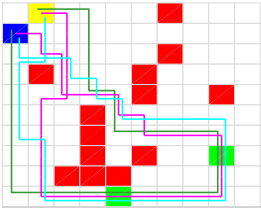
We illustrate our approach on a path planning task in a 10-by10 grid world map, as shown in Figure 1. Each cell represents a state in M, from which the agent has 4 available actions: up, down, left, and right. States are labeled by their colors: r (red), w (white), y (yellow) and b (blue). The two green states are labeled as g1 (green1) and g2 (green2). The yellow state is an absorbing state, i.e., it has no outgoing transitions.
The specification task is to visit both green cells (intermediate goals) in any order, and end at the yellow cell (final goal), while avoiding red cells (obstacles). These requirements are encoded as the co-safe LTL formula ϕcs = ϕinit → (ϕsafe ∧ ϕgoal), where
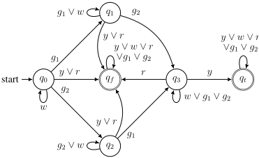
ϕgoal = ((¬y) U ( Fg1 ∧ Fg2)) ∧ ( Fy) (Goal reaching). An equivalent DFA is shown in Figure 2. Each state in the DFA corresponds to some task status (see Table 2), and each transition represents some progress toward task completion. These transitions can be automatically encoded into features to facilitate learning. In fact, three features were constructed this way (see f2, f3, f4 in Table 1). The other two features come from transitions observed in demonstrations (f1), and a penalty for each transition (f5). Note that the final state has no outgoing transitions, and outgoing loops have zero reward.
The agent is given a set of demonstrated trajectories that successfully implemented the task, as shown in Figure 1. In this example all demonstrated trajectories start from the blue cell, pass both green cells (in arbitrary order), avoid all red cells, and eventually end at the yellow cell. States in the upper right corner are never observed in demonstration.
We now discuss the learned policy in three different cases, where the agent is provided with a different amount of side information, and the policies are learned with or without highlevel task information.
Case 1 (MLIRL in M) The agent only knows about the MDPM, the labeling function L, and the demonstrations D, and learns a policy with MLIRL, i.e., by minimizing J mle (θ | M,D) in Eq. (4) while satisfying the constraints (2) and (3).
| Feature | Explanation |
|---|---|
| f1 | f1(s, a) = 1 if (s, a) appeared in demonstra- tion; otherwise f1(s, a) = 0. |
| f2 | f2(s, a) is the probability to reach qt for the first time by taking a at state s. |
| f3 | f3(s, a) is the probability to reach q2, q3 for the first time by taking a at state s. |
| f4 | f4(s, a) is the negative probability to reach red states. |
| f5 | f5(s, a) = -1 if s ̸∈ ¯ SF . |
| DFA State | Interpretation |
| q0 | None of g1, g2, y or r visited. |
| q1 | Visited g1, never visited g2, y, r. |
| q2 | Visited g2, never visited g1, y, r. |
| q3 | Visited g1 and g2, never visited y, r. |
| qt | Visited g1, g2, y without visiting r (success). |
| qf | Visited r, or visited y before visiting both g1 and g2 (failure). |
Since the agent does not know ϕcs or the DFA, we cannot use all features from Table 1. Instead, we replace f2(¯ s, a) and f3(¯ s, a) by the probability of reaching the yellow state or a green state from ¯ s by taking a. All other features have the same interpretation as in Table 1. The learned feature weight vector is
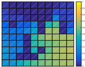
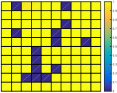
The sign of the learned weights is instructive: they define a policy that seeks to follow demonstrations (f1) and tries to reach the yellow state (f2) in a timely manner (f5). As the weights of f3 and f4 are negative, the agent fails to realize the importance of visiting green states and avoiding red states. There are at least two reasons for such behavior. First, as there is a feature (f1) marking the state-action pairs observed in demonstrations, the agent may simply try to follow the demonstrations whenever possible to minimize J mle (θ | M,D), without further reasoning about the demonstrations, which results in overfitting. Second, there is no side information for the agent to evaluate its policy or identify important features. As shown in Figure 3a, the agent behaves best in the lower right region, where it can follow some expert expert demonstration easily; it behaves the worst in the upper middle region, where the expert demonstrations are lacking.
Case 2 (MLIRL inMϕcs ) The agent has all inputs in Case 1 and the DFA, and learns a policy with MLIRL within the product automaton. Compared with Case 1, the agent can now construct a product automaton. With the extended state space, the agent may behave differently based on the current status with respect to intermediate goals and potentially learn the importance of avoiding red cells. A simple check of the structure of the product automaton reveals that any visit to a red cell will lead to a transition to qf in the DFA, which makes it impossible to reach ¯ SF later. Therefore in order to reach a final state, it is necessary to add some penalty on visiting red states. The learned feature weight vector is
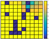
As shown in Figure 3b, the probability of satisfying ϕcs has been greatly improved. The weight for f3 is away from zero as expected, but the weight for f4 is still small, which suggests that the agent still has not learned to always avoid red cells. As a result, the probability of task success is the lowest in the upper right region, which is not covered by demonstrations. The two sources of problems explained in Case 1 still exist
0
0
(c) Policy with augmented objective (Case 3). Min prob: 0.962; average prob: 0.999.
Figure 3: Probability of satisfying ϕcs when following the corresponding policy from each initial state.
here, which calls for the augmentation of objective function using LTL side information.
Case 3 (Policy with augmented objective) The agent has the same input as in Case 2, but now the policy is learned with the augmented objective function J side in (6), where we set g(¯ y) = ∑¯ s∈ ¯ S ¯ y(¯ s | πθ), i.e., the sum of probabilities of satisfying ϕcs from all initial states. With µ = 0.01, the learned feature weight vector is
Compared with ˆ θ(2) , themost significant change in ˆ θ(3) is that the weight on f4 is almost as large as f1, and much larger than the weights on other features. The agent now learns the importance of avoiding red states, and the performance with respect to task implementation has been significantly improved, especially from states that demonstrations fail to cover, as shown in Figure 3c. It shows that, by evaluating policies with side information ϕcs, the agent manages to get rid of the overfitting problem and the induced policy can now be generalized well into regions not previously seen in demonstrations.
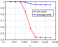
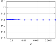
To check the effect of the weight µ, we solved Case 3 with a series of µ and plotted the corresponding minimum and average probabilities of satisfying specification from all possible initial states, and corresponding negative log-likelihood of demonstrated trajectories (see Figure 5). Each experiment is repeated three times. Note that the value of the original objective J mle (θ | Mϕcs ,D) is only slightly affected by µ, while the average probability of satisfying ϕcs is very sensitive to µ. This confirms that the augmentation of the objective function with LTL side information is necessary.
If the given high-level task description is incomplete or inaccurate, as is often the case in practice, demonstrations can compensate for an imperfect specification as long as the features are expressive enough, and no extra memory is needed to implement the missing part of the task.
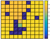
To illustrate this point, we learned a policy where the side requirement to avoid red cells ϕsafe is missing, and evaluated it with respect to the true task encoded by ϕcs. The result is shown in Figure 4. We observe the overall performance is only slightly worse than the case with accurate high-level task information, which suggests that the agent manages to learn from expert demonstration to avoid visiting red states at most initial states. Still, performance can be significantly worse at states that are close to obstacles, such as the cell in row 7, column 5. This example illustrates the agent's ability to learn actions preferences from demonstrations. However if the inaccurate high-level task information leads to insufficient memory states, the performance of the learned policies can be poor, as it is impossible to recover enough missing memory states from demonstration purely by learning the rewards.
6 Conclusions and Future Work
We formulated the problem of IRL with high-level side information on task requirements encoded as co-safe LTL formulas. We proposed two steps to improve the performance of the learned policy with respect to the probability of successfully implementing the task: the first is to construct a product automaton with the original MDP and an equivalent DFA of the co-safe LTL formula, and the second is to augment the objective function by evaluating the probability of satisfying the task requirements. We showed with a path planning example that the induced policy benefits from high-level side information with significantly better performance with respect to the task, especially in regions with few demonstrations.
This work can be extended in several directions. First, algorithms that can account for large state spaces are of interest. Another extension is to consider cases where high-level task requirements are imperfect, for example, if part of the requirements is missing in the high-level specification.
@inproceedings{ijcai2017p426,
  title     = {Learning from Demonstrations with High-Level Side Information},
  author    = {Wen, Min and Papusha, Ivan and Topcu, Ufuk},
  booktitle = {Proceedings of the Twenty-Sixth International Joint Conference on
               Artificial Intelligence, {IJCAI-17}},
  publisher = {International Joint Conferences on Artificial Intelligence Organization},
  editor    = {Carles Sierra, IIIA-CSIC},
  pages     = {3055--3061},
  year      = {2017},
  month     = {8},
  note      = {Main track},
  doi       = {10.24963/ijcai.2017/426},
  url       = {https://doi.org/10.24963/ijcai.2017/426},
}
TY - CPAPER TI - Learning from Demonstrations with High-Level Side Information AU - Wen, Min AU - Papusha, Ivan AU - Topcu, Ufuk T2 - Proceedings of the Twenty-Sixth International Joint Conference on Artificial Intelligence, IJCAI-17 PB - International Joint Conferences on Artificial Intelligence Organization PY - 2017 SP - 3055 EP - 3061 DO - 10.24963/ijcai.2017/426 UR - https://doi.org/10.24963/ijcai.2017/426 ER -Copied
Machine-readable versions of this paper, for tools and AI agents:





